dbMap/Web – Basin Analysis
The basin analysis screen is used to visualise production data for fields and wells, allowing trends in the data to be observed. There are also options to provide forecasts and to compare the production data with prospective values from PLDB.
Field Size Distribution (FSD)
An FSD plots the production values for a set of fields showing how the values are distributed.
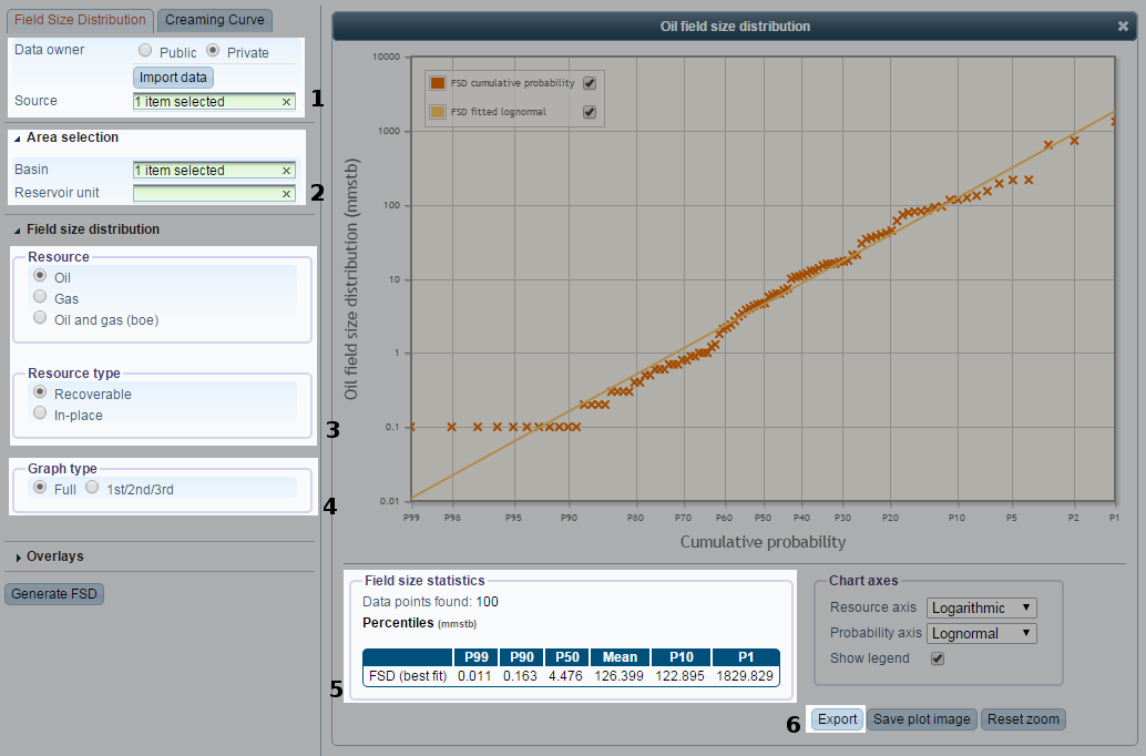 Click to Enlarge | |
1. Data type selection |
Select the type of data to analyse. Private data is only visible to the current user. New data can be uploaded using the Import data option. |
2. Data area selection |
Select the basin(s) and reservoir unit(s) to analyse. If left blank, data from any basin/reservoir unit will be included. |
3. Resource selection |
FSDs can be generated for recoverable or in-place oil, gas and the sum oil and gas (in BOE units). |
4. Graph type |
If the 1st/2nd/3rd option is selected, the data will be split into thirds by date. Each third will have its own separate FSD plotted on the chart. |
5. Summary statistics |
Shows the percentile information for the lognormal best fit of each of the plotted series. |
6. Export |
Exports the FSD data to Excel or CSV. This does not include data from overlays. |
FSD Overlays
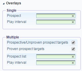
Overlays add additional series to the results view using data from PLDB, which can be compared with the production data. Overlays compute the sum of the target resources for a single prospect and play interval. In most cases, this will be just a single target.
For a “Single” overlay, a prospect and/or play interval must be selected. The full probability distribution for the selected resource is plotted. Only exploration targets are included when computing the data for the overlay.
A “Multiple” overlay requires a prospect selection list and/or play interval. A point is plotted for the mean value of each prospect in the list, limited to the play interval if specified. The type of targets to include in the overlay can be limited by uncheck one of the checkboxes.
Creaming Curve
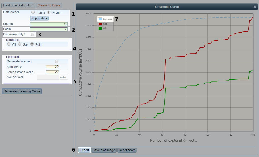
Creaming curves are designed to show the trend in per-well production volumes within a basin over time. This can be used to predict future production. Since larger discoveries within a basin become less likely over time, it can also give an indication of the undiscovered volume within the basin.
 Click to Enlarge | |
1. Data type selection |
Select the type of data to analyse. Private data is only visible to the current user. New data can be uploaded using the Import data option. |
2. Data area selection |
Select the basin(s). If left blank, data from any basin will be included. |
3. Discovery only |
If checked, only non-discovery wells will be ignored. |
4. Resource selection |
Creaming curves can be generated for oil, gas, or both. If “Both” is selected, the oil and gas series are stacked, so that the distance from the x-axis to the green line represents oil volume, the distance between the green and red lines represents the gas volume and the distance from the x-axis to the red line represents the sum of oil and gas. |
5. Forecast |
Generates a forecast based on the trend in the historical data. |
6. Export |
Exports the creaming curve data in Excel or CSV format. |
7. Optimum |
This curve shows the same data as the other series in the creaming curve, but orders the data points by volume (largest first), rather than date, which represents the “ideal” ordering. |
Forecast
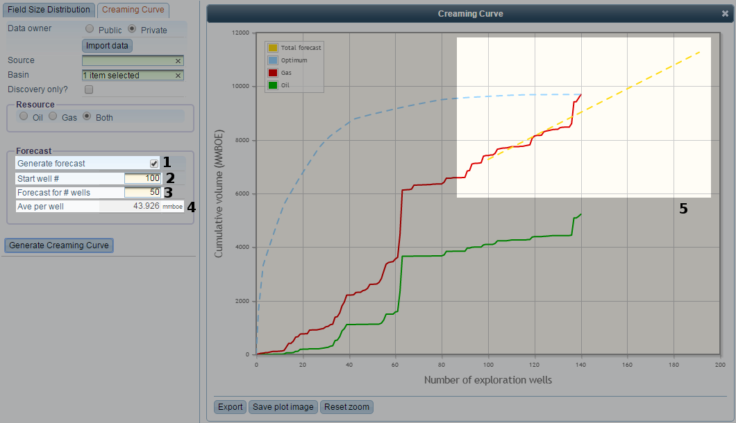
Generates a line of best fit through existing data points to yield a projection into the future.
 Click to Enlarge | |
1. Generate forecast |
Select this option to add a forecast to the results view. |
2. Start well # |
The start well and all later wells will be used to generate the forecast. To use all of the points for the forecast, the start well should be 0. Usually, however, a subset of the points should be used. |
3. Forecast for # wells |
Specifies the number of future wells to forecast for. |
4. Avg per well |
The slope of the forecast line. This is the expected volume for each future well according to the forecast. |
5. Forecast line |
The line of best fit is plotted on top of the creaming curve. It extends back to the specified start well and forwards from the last creaming curve data point for the specified number of forecast wells. |
Data Import
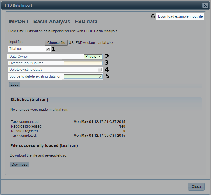
The Import data option provides the ability to upload new public/private production data for both FSDs and creaming curves. Specific options are described below.
 Click to Enlarge | |
1. Trial run |
Simulates the import to generate statistics but does not actually make any changes to the database. |
2. Data owner |
The data can be imported as public – visible to all users, or private – only visible to the current user. |
3. Override input source |
Override the SOURCE value in the input file with the specified value. |
4. Delete existing data |
Delete any data that exists for the specified owner before running the import. |
5. Source to delete existing data for |
Only delete rows that have the specified value for their SOURCE. Only applicable if the “Delete existing data” option is applied. |
6. Download example input file |
Download a template .xlsx file in the correct format for import. This file can be populated with data and then used as the input file for the import. |
Example Input File
As well as list of columns, the example input file (6. above) contains information about each column and whether or not it is required for the import to be successful. Optional columns are colored green, while required columns are blue. In some cases, at least one column in a particular set must be populated. For example, the FSD import does not require all resource types to be populated, but at least one must be populated. This information is available in the comments on the header cells in the example input file.
