dbMap/Web – PLDB Dependencies and Correlations
There are two distinct types of dependency that are used in PLDB:
Risk Factor Dependency – Used to define shared risks between targets. For example, “if Seal of Target A fails then the Seal of Target B must also fail”.
Variable Dependency (Correlation) – Used to define relationships between input variables in a resource computation. For example, “when Porosity is high, it is likely that water saturation will also be high”.
User Interface

PLDB supports dependency of failure between targets. For example, if Target B is said to be 100% dependent on Target A, it means that if Target A fails, then Target B will definitely fail. This is an example of full dependency. A special case of full dependency is total dependency, which means that if either target succeeds, the other will succeed and if either fails, the other will also fail.
PLDB also supports partial dependency, which is weaker than full and total dependency. A partial dependency makes it more likely for targets to fail at the same time, but it is still possible for either target to succeed when the other fails.
Dependency can be applied for any of the prospect risk factors (e.g. Closure, Reservoir, Seal, Charge)
Dependency groups
To create a dependency you first create a group and specify the probability factor (e.g. Closure). You can then add the targets that share a dependency for the chosen probability factor.
The shared probability determines how strong the dependency is. This value must be greater than or equal to the largest independent value of any target in the group and must be less than or equal to 1.
A shared probability of 1 means that there is no dependency and the dependency group will have no effect.
A shared probability equal to the greatest independent target probability means that there is a full dependency.
Any value between these extremes results in a partial dependency.
Technical details
The following example shows two targets A and B, with a partial dependency on the Seal of the targets.

For a partial dependency, all of the individual probabilities are less than 1. This means that there is a chance of each target failing even if the other targets succeed.
The next example shows the same two targets with a full dependency on Seal:

Here the individual probability for target A is 1. This is stronger than a partial dependency and can be expressed as: “If the Seal of Target A fails, then the Seal of Target B will definitely fail”. Note that if the seal of target B fails, then the seal of target A can either fail or succeed.
Finally, if the independent probabilities of the targets are equal, then it is possible to define a total dependency:

This is the same as a full dependency, except that since the independent probabilities are equal, both of the individual probabilities will equal 1. This means that the implication seen in full dependency goes in both directions: “The seal of Target A will fail if and only if the Seal of Target B fails”. In other words, targets A and B have the same seal, so if it succeeds (or fails) for one target, then it must also succeed (or fail) for the other target.
Dependencies are only used when combining multiple targets together to compute total resource values, or rollups, for a prospect, drilling opportunity, play, etc. Resource values for individual targets are unaffected by dependencies.
The effects of applying dependency can be rather subtle and are not always intuitive. The following statements summarise the major implications of adding a dependency while keeping all other parameters the same:
The chance of all targets failing increases
The chance of all targets succeeding also increases.
The overall chance of any success (A or B or Both – the opposite of 1.) decreases
The mean resource for the success case increases.
The mean risked resource is unchanged (risked mean = success case mean * chance of success)
Variable Dependency “Correlation”
This kind of correlation applies to the input variables that are used in resource computation for individual targets. Normally, all input variables are assumed to be independent of one another, so given two variables A and B, a high value for A does not say anything about the value of B. In reality, however, A and B might actually depend on some other factor not explicitly included in the computation, so a high value of A might mean that it is very likely that B will also be high. Correlation values are used to define this sort of relationship.
By default, any pair input variables can have a correlation value as long as neither of them has the “Constant” distribution type. Specific pairs of variables can, however, be configured to disallow correlation values from being specified between them.
User interface
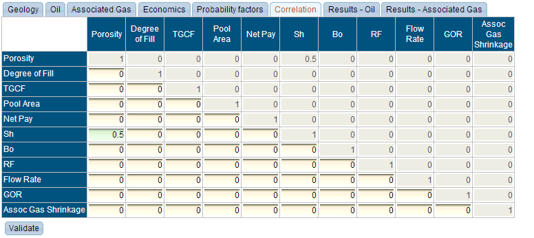
The top-right half of the table is read-only, since only one correlation value can be entered for a pair of variables. Not all combinations of correlation values result in a meaningful scenario. By clicking the “validate” button, you can check to see if the matrix of correlations is valid. If it is not valid, you will see an error message:
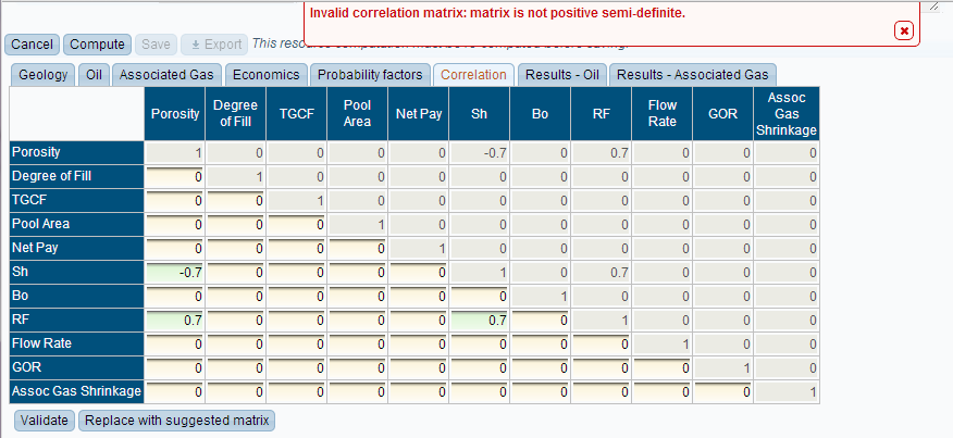
If the matrix is invalid, then you will have the option to replace it with a valid one that is close to the one you entered. If no valid matrix can be found, then this option will not be available, and you will have to change the values manually.
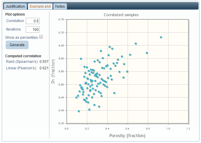
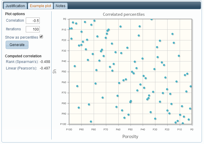
When hovering over a cell in the table, the “information” icon (a small black circle with the letter “i” inside) is shown. Clicking on this icon allows you to enter a justification and notes for a correlation value, as well as seeing an example cross-plot that shows the effect of the correlation value on the two distributions. In this case, there is a moderate correlation between Porosity and Hydrocarbon Saturation, so that if the porosity value is high (or low), then the hydrocarbon saturation value is likely to be high (or low) as well:
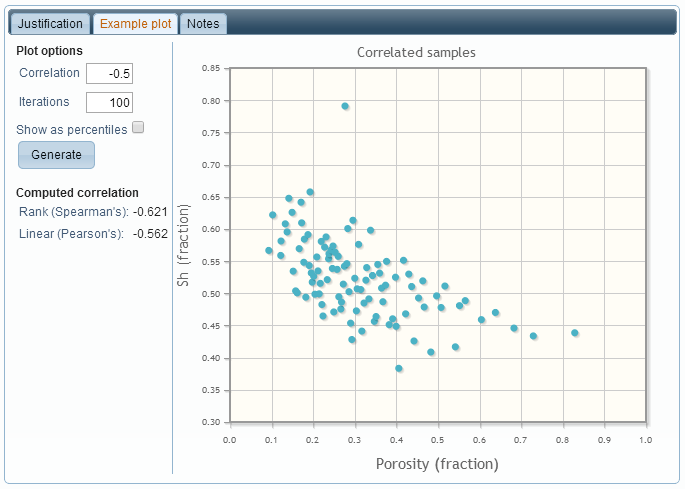
Specifying a negative correlation value means that high values of one variable are likely to occur with low values of the other, and vice-versa:
With the “show as percentiles” option enabled, the cumulative probability is shown, instead of the actual value. This normalises the plot, removing the effects of the distributions:
Resultant effect
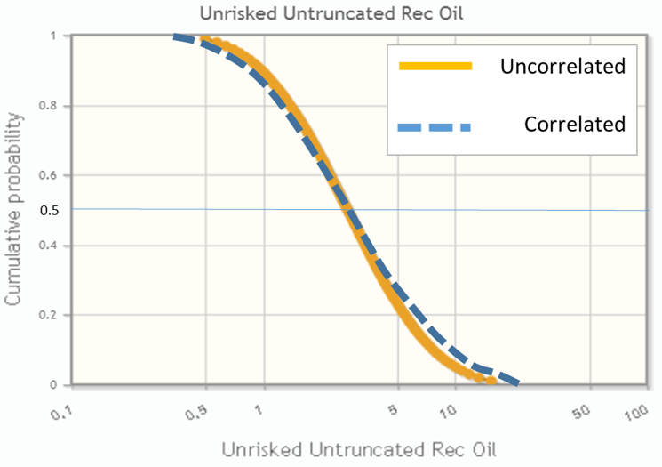
The basic effect applying a positive correlation between two variables A and B has on the output A*B is that the output distribution will be more spread out – the median remains unchanged, but low values will be lower (since low values are likely to occur together) and high values will be higher (since high values are likely to occur together). The mean value will increase. With a negative correlation, the output distribution will be more condensed, since low values in one distribution are likely to occur with high values in the other distribution, with the mean value decreasing and the median remaining unchanged.
Technical details
In reality, not all of the input variables will be independent of one another. For example, it is well-known that porosity and hydrocarbon saturation are very closely related. The correlation between two variables A and B can be thought of as the degree to which A and B vary together. So if A and B are strongly correlated, then for a particular iteration, if the value from A is high, it is likely that the value from B will also be high.
Two common approaches to quantifying correlation are Pearson’s linear correlation and Spearman’s rank correlation. Both produce a single scalar value that describes the correlation between two variables. The former is basically how closely a cross-plot of the variables approximates a straight line and the latter is how closely it approximates an increasing (monotonic) function.
In PLDB, the user enters the desired value between 0 and 1 for a pair of variables, and the generated samples will be such that the Spearman’s correlation approximates the given value. The Pearson’s correlation will likely be similar, but this is not guaranteed, especially for very skewed distributions.
The approach used in PLDB is similar to the Gaussian Copula method, except for the fact that the original samples are retained, and re-ordered based on the generated correlated sample.
Correlation does not affect the actual distributions of the individual variables (known as marginal distributions). The way that correlation is imposed is to re-order the sample values from the distributions, so that the desired correlation coefficients are (approximately) obtained, without modifying the distributions or the latin-hypercube properties of the sample.